Showing posts with label R. Show all posts

Sunday, July 29, 2012

Pre-allocate your vectors

Or else welcome the good ol' friend, the O(n^2) back in your life.

There are three common ways people add elements to vectors in R. First way:

f1 <- function (n) {
    l <- list()
    for(idx in 1:n) {
        l <- append(l, idx)
    }
    return(l)
}

This is bad. It does what it looks like: adds one element to the vector and then copies it to another variable, which just happens to be the same variable 'l'. This is clearly O(n^2).

The second method is this:
f2 <- function (n) {
    l <- list()
    for(idx in 1:n) {
        l[[length(l) + 1]] <- idx
    }
    return(l)
}

This approach looks decent because, coming from a Python and Java background, a good implementation would allow appending elements to vectors in amortized O(1) time. However, this holds an unpleasant surprize. Another good ol' O(n^2) in lurking in the shadows here.

Time taken to create a vector of size n
The method f2 is arguably better than f1, but none of them is any match for f3 which simply uses pre-allocation:

f3 <- function (n) {
    l <- vector("list", n)
    for(idx in 1:n) {
        l[[idx]] <- idx
    }
    return(l)
}


Of course these are just cooked up examples, but it is not difficult to imagine situations where such incremental creation of list is inevitable (think reading from DB cursors). For this particular example, the fastest solution involves a sapply but is not much faster then f3:

f4 <- function (n) {
    return(as.list(sapply(1:n, function (idx) idx)))
}

So in most cases it'll be better to overestimate the number of items in a list and then truncating it to the right size than dynamically expanding it.

And don't forget to smile and wave at the hidden O(n^2)!

~
musically_ut

PS: If you want to run the profile yourself, here's the gist of the functions and the profiling code.
Colors in R console

Update 2: The colorout package has moved again and is now available on GitHub.

install.packages('devtools')
library(devtools)
install_github('jalvesaq/colorout')

Update: The colorout package on CRAN has not been updated to be compatible with R version 3.x.x yet. However, if you compile and install it yourself, it still works.

download.file("http://www.lepem.ufc.br/jaa/colorout_1.0-1.tar.gz", destfile = "colorout_1.0-1.tar.gz")
install.packages("colorout_1.0-1.tar.gz", type = "source", repos = NULL)

 R console


Let's face it, the R-console is one of the more uninviting things I have seen, perhaps second only to the Ocaml console which comes without readline.

This is what my (and probably your) R console looks like this:
R console without color
What I see on the console is a single color which, firstly, makes it a challenge to separate stderr, output, warnings and errors, and, secondly, is just boring. I did not know what I could do about it and I stuck with it because the only other option seemed to be moving to a GUI (JGR or Rstudio). This is not to say that there is something wrong with the GUIs, but I prefer working with only my keyboard and, hence, shun GUIs almost as a rule. (Eclipse for Java is an exception.)

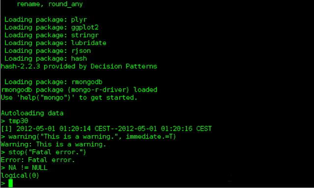
But it changed when I discovered the package colorout on CRAN, which makes my console look like this:
R console with color (using colorout)
This makes it remarkably easier to differentiate different forms of output.
The coloring is not perfect (notice that the second '-' in the interval outputted for tmp30 is assumed to be a negative sign instead of being a separator), but I would choose it any given day over the drab single color.
I did need a little tweak to my .Rprofile file since I did not like the way the default settings display the error:

~
musically_ut

Saturday, November 26, 2011

Handling NULLs and NAs

Real world data always has missing and blatantly incorrect values.

This becomes a painful issue when it comes to coming up with predictive models. While there are multiple ways of imputing data, it is difficult to figure out whether one is doing a good enough job. To make matters worse, the rows missing data might not be random. For example, all incomes above a certain threshold might be deliberately made NA to preserve anonymity. However, the model developer might not be aware of this censoring. Imputing data using any central measure will not only fail to capture this bit of information, but will actually make predictions worse.

Similar encoding might be present when one sees columns with values outside the natural limits. For example, say a column that contains number of questions answered from 5 questions in a test having the value -1 to indicate absentees.

In the worst case, a model developed by completely dropping the offending parameter might perform better than an imputed data-set.

In most cases, we can do better.

Wednesday, October 19, 2011

Humble "FrozenSynapse" Bundle

Humble Bundle came back again, this time with just one new game FrozenSynapse and the previous FrozenByte bundle with it, if you paid more than the average.

This run of the Bundle was not as peppered with events as the previous bundles were: there were only two mid-air additions to the bundle, instead of half a score of interesting events happening the last time and nothing (to the best of my knowledge) was made open source:

Humble "FrozenSynapse" Bundle's economic performance

Sunday, September 11, 2011

What Perl got right and R got wrong

R tries to do the right thing by having very short names for functions one uses often:

c()
Creating vectors.
t()
Transpose a matrix.
q()
Quitting R
is()
Generic isInstanceOf
by()
apply after grouping
as()
Generic type cast
Common primitive functions in R

As much as I like not having to type extra characters to get to these functions, I have always had to be extra cautious when it comes to naming my variables out of fear of accidentally overwriting any of these. Interestingly, R selectively ignores such overrides letting the primitives prevail if possible:

> R.version.string
[1] "R version 2.12.1 (2010-12-16)"

> c <- function(...) { 42 }   # Accidentally overriding c()
> c(45, 67, 78)               # Expected behavior
[1] 42

> c <- "42"                   # Now it should be a scalar, right?
> c
[1] "42"

> c(45, 67, 78)               # Magical return from the dead!
[1] 45 67 78

This overriding of an identifier as both variable and primitive function is grossly inconsistent, specially since functions are first class objects, same as any vector or string. If I override an identifier, even a primitive, I expect it to be really overridden.

Though the intention of cutting keystrokes is clearly good here, this inconsistency feels avoidable.

On the other hand
In contrast, this highlights how well Perl does the same thing. Larry Wall, the creator of Perl, was a linguist by education and one of his tenets while creating Perl was making it as succinct as possible. To this end, it ventured to those corners of the keyboard which only APL had gone beyond. Also, on an unrelated note, he was the winner of the International Obfuscated C contest twice and some say that after Perl became mainstream, there wasn't much point left in obfuscation contests.

Perl also short-cuts most commonly used functions and type qualifiers:

my
Variable definitions
@a
Array variable prefix
%a
Hash variable prefix
$a
Scalar variable prefix
s//
Substitute function
m//
Match function
Common primitive functions in Perl

However, in Perl, the domain of the abbreviations looks completely different from identifiers; it is impossible to even imagine confusing them. In R, the use of identifiers and built-in primitives seems uniform, and is actually inconsistent.

And we have a winner ...

I think between R and Perl, Perl is the one which got it completely right.

The design principle to be learned here perhaps is that of having different keystrokes for different folks. The onus of preserving the (abbreviated) primitive functions should lie with the language, and it can be done:

  • the right way by syntactical obviousness as Perl does it,
  • the good ol' way by reserving keywords as Python does it or,
  • the wrong way by allowing overrides and resuscitating primitives as R does it.


Wednesday, August 31, 2011

R: Going faster than vectorization

Introduction

Update: The by function of R can be used for the same task since data for me is stored in the same data.frame. I have tested that out later on in the post.


Recently I had to run though a large data.frame in R, selecting values from a given column based on an equality constraint on another column, in this format:

for(i in 1:length(values)) { 
  t <- my.var$row2[ my.var$row1 == value[i] ]; 
  do.something.interesting(t); 
}

This is a fairly common operation and I had thought that beyond the vectorization I had done (borrowed term from MATLAB), R would take care of optimizations under-the-hood.

At this point, I thought how I would do it on a larger database and it struck me that perhaps I can do better than R if I manually index the data and find relevant intervals myself. How much faster can that be?

Wednesday, August 10, 2011

Humble Indie Bundle 3: A review

It was jolly good ride for the Humble Bundle 3, and it was far better and more exciting in the second half than the first one:
15 days of Hunble India Bundle 3

Wednesday, July 27, 2011

HumbleBundle is back again!

And this time, I am not late!

Err ... not very late anyhow. I did miss the action for the first $40,000 but got around to collecting data much faster than the last time around. If you do not know what a HumbleBundle is, read the wikipedia entry, or just visit their website here.

The start of the action is explosive!
The amount raised by the Humble Indie Bundle 3 so far, in minutes since my 1st data reading
(14 more days to go)


Thursday, July 14, 2011

Tough times for Geneva

Lurking though the data for number of companies which declared bankruptcy in Geneva (data available from here), I noticed something:


So, as soon as I left for my internship in Japan in July '10, things headed down. They hit rock bottom in October 2010 and improved spectacularly in March '11, the month I landed back in Switzerland.

Something was up in Geneva while I was not here (July '10 - Feb 11).

Just sayin ...


~
musically_ut

PS: I was a little sad to see 27 business close doors on 24th December, 2010 and 15 businesses on 23th December, 2009.

Saturday, July 9, 2011

Debugging puzzle in R

Here's a small debugging puzzle in R. I recently came ran into it and thought that the bug was rather elegant. I have simplified down the problem I faced, but not all the way to keep a little fun in.

Explain the output
>> # a is a (large) vector with numerical elements
>> any(is.nan(a))
[1] FALSE

>> any(is.nan(exp(a)))
[1] FALSE

>> any(is.nan(exp(1.0 * a)))
[1] FALSE

>> any(is.nan(exp(0.0 * a)))
[1] TRUE

See something surprizing? Suddenly a NaN where there was none before?

Can you think why this is happening?

Hint
If you give up, then click-and-drag to select and see the hint below:

>> # Multiplying an Infinity with zero gives a NaN
>> Inf * 0
[1] NaN


~
musically_ut

Saturday, May 7, 2011

Declaring software open-source considered helpful

There have been two Humble Bundles released in the last six months:

  1. Humble Indie Bundle in December, 2010
  2. Humble Frozenbyte Bundle in April, 2011
The summary statistics themselves are enough to challenge some established stereotypes, e.g. the average amount contributed by Linux users has consistently been significantly larger than the Mac OS or Windows counterparts, showing that Linux users are willing to pay more than non-linux users for quality software.

On a larger scale, considering these to be real-world economic experiments, there is still much information buried deeper in the data than can be gleaned by looking at the summary. Here, I look at five-minute sampled data to see what effect making the software open-source had on the sales:

Contribution and purchases data for the Humble Frozenbyte bundle.
The projections show what the contributions and purchases might have been if Frozenbyte had not declared their games open source.

Sunday, December 12, 2010

Are Firefox sessions are really this short?

I have been meaning to play with the Test pilot data for quite a while now. The primary problem was, err ..., my Harddisk space.

Anyhow, I got the data downloaded finally, only to see that my computer's memory was the next bottleneck. Things looked hopeless till I started looking at it as an exercise in online algorithms.

Then I saw one thin silver lining: the data in the csv file was presorted by the user_ids.

There was my window! If I could pre-segment the data based on the user-ids, then I could run though one user at a time, instead of reading all the data. Though not much, but linear grouping of the users already saved me a lot of effort. My next hope was that after ordering by the user ids, the data would be ordered by timestamps. Sadly it wasn't, but one cannot have everything in life anyway. :-)


  • Extracting the data

After a quick perl script to confirm the ordering of user_ids, I wrote a script to calculate the time intervals between a BROWSER_STARTUP event and a BROWSER_SHUTDOWN event in the data. There were various instances when the BROWSER_STARTUP event was present without a BROWSER_SHUTDOWN event. Probably the browser was started when the system was online (most uses of Firefox are online, after all) but the system was not online when the browser was shutdown (or crashed). So, I skipped all the orphaned start-up events. Also, some startup-events might also be made while the host was offline, and ignoring these would bias the intervals towards being longer.  I cleaned up the data (there were a few instances ~ 10s when the session lasted beyond 7 days?) and I plotted the intervals (on a semi-log scale) in R.


Now I am a user who generally carries his laptop around and has his browser open almost all the time. I was in for a small surprise, enough to make me go over the code twice before I realized that the code was correct and my intuition was wrong.

  • Visualizing the data

This data extraction took a whopping 30 minutes on my meager laptop. The stats are here (all numerical values in milliseconds):


Maximum interval = 534616265 ms  (6 days)
Minimum interval = 31 ms
Mean = 4286667.42334182 ms (1.1 hours)
Median = 896310ms (15 minutes!)
Skipped 54748 out of 633212 BROWSER_STARTS


50% sessions were less than 15 minutes long, and this is while the intervals are biased to be longer!


Of course, there are some very long periods, which pull the mean up to 1 hour, but considering that there might be outliers in the data, median is a far more robust measure. In case it is not apparent, this is a beautiful log-normal distribution staring one in the face.

It took me a while to imagine that most operations with a browser end rather quickly for most people, they do not live their lives in a browser. In other words, I am an outlier here!


How long do Firefox sessions last?

  • Conclusion

I am sure most people at Mozilla know this and, if this is indeed correct, they probably are making sure that Firefox is well suited for short operations and not extended week long uses. I am not sure whether these are competing demands, perhaps making the start-up quicker, pre-indexing search files, etc. also help in extended sessions. However, it appears (with more than just a pinch of salt) that Firefox should focus on the quick-draw and fire users for gaining market in the short term, at least. This is taking the exact opposite direction of Chrome's development, by the way.

However, there are alternate explanations possible. I am not sure how many of these were voluntary terminations; it might be that these are regular restarts. Or it might be an indication of a bigger problem, as this comment indicates:  frequent cold-restarts forced by the user to reduce the memory footprint of the browser. Or it might be that people are using Firefox only as a compatibility browser, when something (like Java applets, or broken Javascript code for example) does not work correctly on other browsers, they fire up Firefox, do the task and return back. This last question can be answered using the Survey data.

Will keep digging and hoping to find something interesting.

Feedback welcome.

Update: A few more important factors are:

  1. What were the average session times per user?
  2. How many Browser sessions were still open when the week ended?
These concerns will be addressed in the newer post.
These have been addressed in this post.


~
musically_ut